
mieardjoune/ecc_scaler_mult · Elliptic curve scalar multiplication over GF(2^233), Modified Lopez-Dahab coordinates, verified against a Python model, reachable over UART
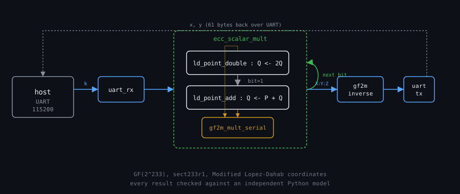
Elliptic curve scalar multiplication is one operation, k times P, and almost the entire cost of any elliptic curve cryptosystem lives inside it. Do it over a binary field like GF(2^233) and every one of the field operations underneath, add, multiply, square, invert, is its own design problem before you’ve even gotten to a single point on the curve. This project is that whole stack built from the ground up: multiplication, squaring, inversion, point doubling, point addition, and the scalar multiplication loop that ties them together, in SystemVerilog, checked against an independent Python implementation of the same math, and reachable over a plain UART link so the answer can come from real silicon instead of a simulator.
Why a binary field, why this coordinate system#
GF(2^233) is the field behind standard curve sect233r1, NIST B-233. Addition is XOR, multiplication is shift-and-add with a fixed reduction polynomial, and squaring is a bit spread instead of a full multiply, because squaring is linear in characteristic 2. None of that changes how expensive point arithmetic gets if you do it naively: plain affine coordinates need a field inversion for every single point addition, and inversion is the slowest operation in the whole stack by a wide margin.
Modified Lopez-Dahab coordinates fix that by deferring the inversion. A point is carried as (X : Y : Z) instead of (x, y), with x = X/Z and y = Y/Z^2, and the “modified” part shaves four more multiplications off point addition specifically for the case where one of the two points being added has Z = 1, which is exactly the situation you’re in when that point is a fixed base point that never gets updated. You only pay for one inversion at the very end, converting the final projective result back to affine.
Two ways to get this wrong#
Working out this exact coordinate system from scratch surfaced two mistakes that are worth knowing about if you’re implementing this yourself, because both are the kind of thing that looks correct until you actually run it.
The first is the final conversion back to affine. The correct formula is y = Y/Z^2, not y = Y. An earlier attempt at this same idea I reasoned that 1/Z^2 = 1 so the division could be skipped and y read off directly as Y. That’s only true when Z happens to equal 1, and after an actual scalar multiplication Z is essentially never 1. Skip that division and you get a wrong y coordinate almost every time.
The second is which point is allowed to keep Z = 1. The Modified Lopez-Dahab addition formula requires one specific operand to stay at Z = 1 permanently. A natural-looking way to write the scalar multiplication loop is to keep doubling the base point itself, bit by bit, while a separate accumulator collects the result. The problem is that after the very first doubling, the point you’re doubling no longer has Z = 1, but it keeps getting fed into the addition formula as if it still did. The fix is to swap which point plays which role: keep the base point fixed at Z = 1 forever, and double the accumulator instead, since the accumulator is allowed to have any Z. That’s a left to right double-and-add instead of a right to left one, same bits, opposite direction, and it’s the difference between an addition formula that’s valid on every call and one that’s only valid on the first.
One multiplier, called a lot#
Every module in src/ shares a single serial multiplier instance rather than running several in parallel. gf2m_mult_serial is a straight shift-and-add multiplier, one bit of the multiplicand consumed per clock, 233 cycles from start to done. Squaring skips the multiplier entirely, it’s a combinational bit-spread-and-reduce, free in cycles. Inversion (gf2m_inverse) is Itoh-Tsujii: instead of ~232 multiplications for a naive Fermat exponentiation, it builds the same result in about 11, by replaying a fixed double-and-increment sequence derived from the bits of 232 at elaboration time.
Point doubling and point addition (ld_point_double, ld_point_add) are each a small state machine wrapped around one multiplier instance, sequencing the field operations from the Modified Lopez-Dahab formulas one at a time. Doubling takes 4 multiplies, addition takes 8, both slower than a parallel datapath would be, both a lot easier to know are correct. ld_point_add doesn’t even expose a Z1 input port, the operand that has to stay at Z = 1 is only ever wired from the module’s X1/Y1 inputs, so the precondition from the bug above can’t be violated by construction, there’s no wire you could connect that would break it.
ecc_scalar_mult is the loop itself: left to right double-and-add, doubling the accumulator every bit and adding the fixed base point in whenever the current bit is 1, then one final inversion and two multiplies to get back to affine coordinates. It also handles the point at infinity explicitly in two places, because the addition formula underneath has no built-in notion of it: k = 0 is reported as infinity without running the loop, and the first time the accumulator has to receive a point while it’s still at infinity, the state machine just loads the base point directly instead of calling the adder with a Z = 0 operand it wouldn’t know what to do with.
Checking it against something that isn’t itself#
python_model/ is a second, independent implementation of the same math, written separately from the RTL and sharing no code with it. It includes a plain affine-coordinate reference implementation with its own inversion per point operation, slow and obviously correct, used to cross-check the projective code on random points. It also keeps the two broken variants around under names ending in _naive, so the mistakes above can be reproduced on demand rather than just described.
Every RTL module has its own Icarus Verilog testbench, checked against fixed known-answer vectors generated by the Python model, right down to reproducing a hand-worked multiplication and division example bit for bit. The strongest one walks a full 233-bit scalar and checks (n-1)*G against -G, which for this curve just needs matching the x coordinate against the base point’s own x, since -P = (x, x+y) here. That test alone exercises every loop iteration, both the doubling and addition paths, and the final inversion, all in one pass.
Getting an answer out of real hardware#
ecc_uart_top wraps the whole scalar multiplier in a small, fixed-length UART protocol at 115200 baud so the design can be tested on an actual board instead of only in simulation. Send 30 bytes encoding a scalar k, big-endian, and the FPGA multiplies it against a fixed base point and sends back 61 bytes: one status byte, then Qx and Qy in the same encoding. The response length never changes, even for the point-at-infinity case, so a host script never has to branch on how many bytes to expect. After replying it goes straight back to waiting for the next scalar, no reset needed between runs.
host/ecc_uart_client.py is a small python serial script that speaks this protocol from the other end, with a --check flag that runs the same scalar through the Python model and compares the two answers automatically. That closes the loop all the way: math worked out independently in Python, RTL checked against it in simulation, and the same vectors checked one more time against whatever the actual chip says over a serial cable.
One bug while we’re here: the reset polarity for the QMTECH board. Nothing catastrophic, results are correct, exactly what you’d expect, just keep pressing the RESET button for an answer.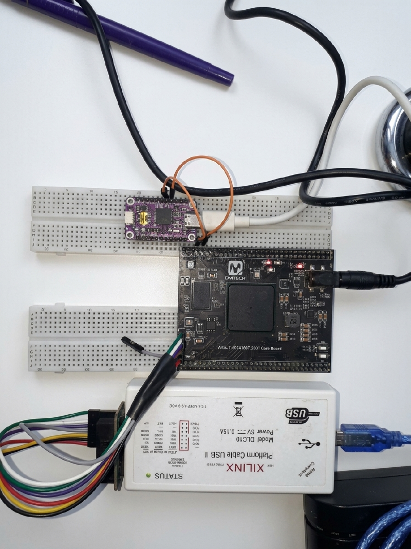
Running it#
make sim PRJ=ecc_scalar_mult        # RTL simulation (Icarus Verilog)
make build PRJ=ecc_scalar_mult      # Synthesis + implementation + bitstream
make sim-gate PRJ=ecc_scalar_mult   # Gate-level timing simulation
make deploy PRJ=ecc_scalar_mult     # Program the board over JTAG
To talk to a programmed board instead:
sudo python3 projects/ecc_scalar_mult/host/ecc_uart_client.py /dev/ttyUSB0 12345 --checkResults#
| Metric | Value |
|---|---|
| Area: Slice LUTs (with UART) | 9,650 (15.22% utilization) — Post-Implementation |
| Area: Slice Registers (with UART) | 15,870 (12.52% utilization) — Post-Implementation |
| Area: Total Slices (with UART) | 3,896 (24.58% utilization) — Post-Implementation |
| Total On-Chip Power | 0.161 W |
| Dynamic Power | 0.064 W |
| Static Power | 0.097 W |
| Target Clock Period | 20.000 ns (50.000 MHz) |
| Worst Negative Slack (WNS) | 4.472 ns (Overall Design) / 7.279 ns (Intra-Clock Setup) |
| Maximum Frequency (f_max) | ~64.40 MHz (Overall WNS) / ~78.61 MHz (Internal logic setup) |
| One Scalar Multiplication Time (Simulation at 50 MHz) | 3.84 milliseconds (192,044 clock cycles) |
| Total Time with UART Overhead (Simulation at 50 MHz) | 13.90 milliseconds (695,109 clock cycles) |
Apache 2.0 licensed.